Instructions

The following learning outcomes will be assessed:

1.    Critically select and apply key machine learning and statistical techniques for data analytics projects across the whole data science lifecycle on modern data science platforms and with data science programming languages.
2.    Appropriately characterize the types of data; to perform the pre-processing, transformation, fusion, analysis of a wide range type of data; and to visualize and report the results of the analysis of various types of data.

Your Task

THIS ASSIGNMENT REQUIRES R CODING AND A SHORT REPORT (65% of module marks)

Your task is to conduct data analysis on a given data set from the UCI site. To help you in this task please look over our past RStudio activities where we loaded in data, pre-processed it, trained machine learning algorithms on the data and plotted the results. 

The first part of the report is simply text describing the introduction, application area and data to be used, machine learning algorithms to be used. 

What I expect to see for the practical implementation part of the report are screenshots of your code in the RStudio script editor. Screenshots of key outputs and screenshots of important diagrams. Along with text to describe what I’m seeing and identify any salient points. The presentation of your practical work should be identical to the way I’ve presented the Activities in R over the last seven weeks.  You need to use snipping tool in Windows or similar to grab screenshots of selected areas. 

Finally, write up your work in a 1,500 word (+/- 10%) report 

1.    Introduction

Your introduction should include a summary of the main points that you will discuss in your report. Your report should outline the area your data is from and what you hope to achieve.  Your introduction should be about 150 words in length.

2.  Data used

The purpose of this section is to ensure you understand the types of data and the pre-processing you will use. What types of variables are present such as: integer, dates, strings, etc.  Provide literature and examples associated with your data set. This section should be approximately 150 words. 

3.    Machine learning methods used

In this section you should identify the machine learning methods that you will apply to the UCI data. What criteria will be used to measure the success of the machine learning methods. This section should be approximately 150 words.

4.    Practical: Pre-processing of data

In this section you should discuss how the data was read in, what pre-processing if any occurred and why you did it.  Show me screen shots of code with your text write up. This section should be no more than 150 words in length.

5.    Practical: R Programming content

In this section you should show me screen shots of code with your text write up. The R programming content can include building your machine learning models, testing of models, perhaps you have done a compare/contrast with several models.  I would also like to see an R function written by you. The source code should be neat and tidy, use comments where necessary to explain the main actions of your code.  This section should be no more than 300 words in length.

6.    Practical: Display of data/results    

This section you should use screenshots of key R output, important diagrams and anything to do with your machine learning models. Along with text descriptions of the outputs. It should be no more than 300 words in length.

7.    Source code listing

This includes all your R code including the library commands. I expect to be able to load in the libraries you have used and copy and paste and run your analysis.

8.    Conclusions

In this section you should summarise your experimental results and findings. This section should be approximately 150 words.

9.    References and look and feel of report

These should be to Harvard standards (not included in work count but should be between 5-10 references). References should be valid and appropriate. The formatting of the report should be neat and tidy. Diagrams should be used with good descriptive text. Diagrams should be easy to read, and a sensible number of no more than 6-7 diagrams used. No more than 15 pages in total for everything including source code listings, put source code listing in font size 10.

Also Read - Visual Studio Assignment Help

1. Introduction

This report examines the application of data science concepts to examine the Breast Cancer Wisconsin dataset, which is considered a foundational dataset in health and medicine. In 1992, the dataset was generously donated; it contains 699 instances with 9 features each emphasizing the characteristics of cell samples.

Its main objective is to use machine learning and statistical methods throughout the data science process to build a model for predicting whether or not breast tumors are benign.

We are going to look into the data's source, its time breakdown, and what form it takes-such as for instance clump thickness, cell size uniformity. The selection of machine learning algorithms, pre-processing steps, and their effects on the data will be considered.

Using R programming, we will highlight how a decision tree model is actually run, as well as assessing its effectiveness. The report concludes with some inferences drawn from the experimental results and possible next steps for breast cancer classification.

2. Data Used

The Breast Cancer Wisconsin dataset includes more than a dozen of the most important variables for defining cell samples in breast tumors.

These variables, mostly integer-based, are clump thickness as well as uniform cell size and shape of the epithelium; marginal adhesion; single epithelial cell size; bare nuclei (without a true cytoplasm); bland chromatin (no visible entity except for masses of residual ribonucleoprotein on mitosis).

The class variable becomes the object, designating whether tumors are benign (2) or malignant (4).

Studies by (Osareh and Shadgar, 2010) , (Yue et al., 2018) , (Amrane et al., 2018), (Aamir et al., 2022), (Khan et Al., 2022), (Kirola et al., 2022), (Farhadi et al., 2019) and (Fatima et al., 2020), among the many literature on breast cancer classification note this importance of these variables in terms of predictive modeling. These efforts highlight the applicability of machine learning methods. Using them one can identify benign from malignant tumors.

In our analysis, for data processing we used R and implemented a decision tree model. In particular, missing values in the “bare_nuclei” variable were temporarily substituted by median imputation.

3. Machine Learning Methods Used

A decision tree model was developed using the rpart method in R to analyze the Breast Cancer Wisconsin dataset. Decision trees are able to handle classification tasks, while at the same time being very intuitive and easy to visualize.

This is especially useful within a medical context. The model was designed to predict whether tumors were being benign or malignant, according to the selected features.

The efficacy of the machine learning technique was measured through various metrics derived from the confusion matrix, including accuracy, sensitivity, specificity, positive predictive value and negative predictive value.

Together these measurements measure the model's ability to accurately classify examples, distinguishing between those that are true positives and false negatives on the one hand and true negatives and false positives on the other.

These measures show us something about the efficiency of this decision tree in its classification of breast cancer.

Also Read - IT Assignment Help

4. Practical: Pre-processing of Data

The first step in the data analysis process was to load the required libraries, including caret and ggplot2. The dataset was taken from the UCI Machine Learning Repository. 

 
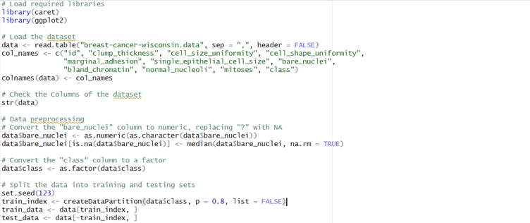
Figure 1 Data Loading and Pre-processing Code

It was read into R through the use of the function read.table(). Names for the columns were then chosen in accordance with the given information. A preliminary examination of the structure of the dataset with str(data) informed that the data in the "bare_nuclei" column were stored as characters. 

 
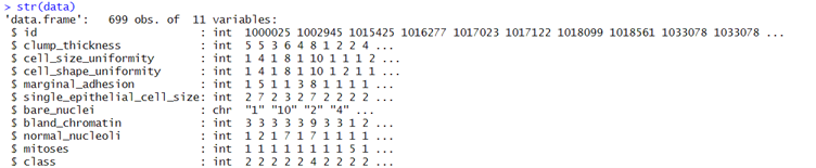
Figure 2 Sample Column values along with their data types

For this purpose, the column was changed to numeric, replacing any "?"s with the median of the column. Also, the category column which differentiates between benign and malignant tumors was coded as a factor to ease model training.

The dataset was then split into training and testing sets, with 80 % of the data used for learning and the remaining 20 % for testing. These operations are pre-processing for data to put it in good shape for applying subsequent machine learning model training and evaluation.

Also Read -

5. Practical: R Programming Content

In this section, we carried out three essential R functions for training and testing the machine learning model. These functions are meant to increase code modularity, reusability and readability. The functions are:


 
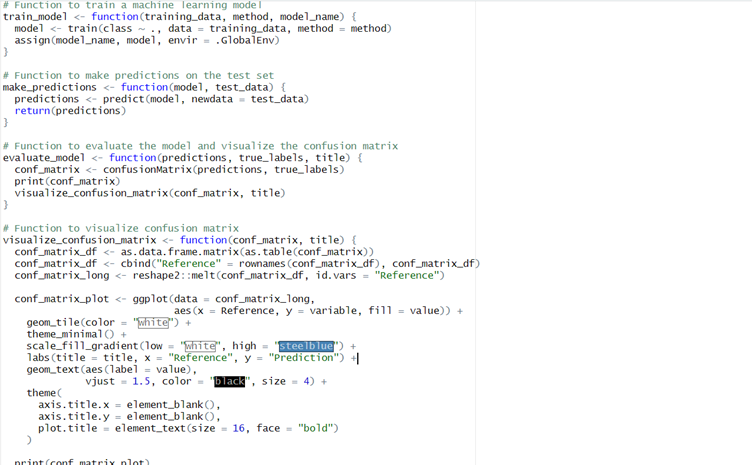
Figure 3 Functions to Train, Predict, Evaluate and Visualisation

1.    train_model function: This function trains a machine learning model using the train function of the caret package. It takes three parameters: training_data (the data set for training), method (machine learning algorithm/technique to be used) and model_name (the name we will assign to the trained model in the global environment).
2.    make_predictions function: Given a trained model and a test dataset, this function makes predictions with the predict function. It returns the predicted values.
3.    evaluate_model and visualize_confusion_matrix functions: These functions perform evaluations of the model using the confusion matrix, and then visualize the results as a heatmap. These Functions take predicted values, true labels and a title for input to evalue and visualise.



 
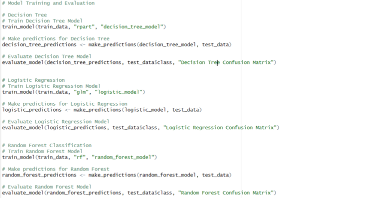
Figure 4 Model Training and Evaluation

Finally, the Figure 4 shows the use of the above functions to train and evaluate three different Machine Learning classifiers which are Decision Tree, Logistic Regression and Random Forest. Each model is trained and then the predictions are made on the test dataset and the corresponding confusion matrix is visualized. Using this structured approach of functions, it makes code easier to read, and to compare different models more easily.

6. Practical: Display of data/results

The Prediction and Evaluations gives Confusion Matrix and Statistics as their output and for each of the three classifiers, Confusion matrix is shown and interpreted. 




  
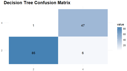
The Results of Decision Tree indicates 94.96 % accuracy and the model shows a sensitivity of 93.41 % which means that it was able to correctly identify positive cases, and specificity of 97.92 % indicating the accuracy with which it identified negative cases. Agreement beyond chance is demonstrated by the Kappa coefficient which had value of 0.8913.

  



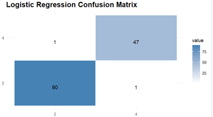
The Next Model to Evaluate and Visualise is Logistic Regression model. It delivers respectable performance with an accuracy of 98.56 %and the confusion matrix shows high sensitivity (98.90%) and specificity (97.92%), showing that the model is good at classifying both positive examples and negative ones correctly. The Kappa coefficient is high with a value of 0.9682 which indicates excellent agreement.




  
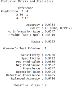
Finally, the Random Forest model also performs well with an accuracy of 97.84% and the confusion matrix indicated a good balance having sensitivity and specificity both over 97 %. Also, The Kappa coefficient for the Random Forest model was 0.9525 which indicated high substantial agreement.

7. Source code listing

# Load required libraries
library(caret)
library(ggplot2)

# Load the dataset
data <- read.table("breast-cancer-wisconsin.data", sep = ",", header = FALSE)
col_names <- c("id", "clump_thickness", "cell_size_uniformity", "cell_shape_uniformity", 
               "marginal_adhesion", "single_epithelial_cell_size", "bare_nuclei", 
               "bland_chromatin", "normal_nucleoli", "mitoses", "class")
colnames(data) <- col_names

# Check the Columns of the dataset
str(data)

# Data preprocessing
# Convert the "bare_nuclei" column to numeric, replacing "?" with NA
data$bare_nuclei <- as.numeric(as.character(data$bare_nuclei))
data$bare_nuclei[is.na(data$bare_nuclei)] <- median(data$bare_nuclei, na.rm = TRUE)

# Convert the "class" column to a factor
data$class <- as.factor(data$class)

# Split the data into training and testing sets
set.seed(123)
train_index <- createDataPartition(data$class, p = 0.8, list = FALSE)
train_data <- data[train_index, ]
test_data <- data[-train_index, ]

# Function to train a machine learning model
train_model <- function(training_data, method, model_name) {
  model <- train(class ~ ., data = training_data, method = method)
  assign(model_name, model, envir = .GlobalEnv)
}

# Function to make predictions on the test set
make_predictions <- function(model, test_data) {
  predictions <- predict(model, newdata = test_data)
  return(predictions)
}

# Function to evaluate the model and visualize the confusion matrix
evaluate_model <- function(predictions, true_labels, title) {
  conf_matrix <- confusionMatrix(predictions, true_labels)
  print(conf_matrix)
  visualize_confusion_matrix(conf_matrix, title)
}

# Function to visualize confusion matrix
visualize_confusion_matrix <- function(conf_matrix, title) {
  conf_matrix_df <- as.data.frame.matrix(as.table(conf_matrix))
  conf_matrix_df <- cbind("Reference" = rownames(conf_matrix_df), conf_matrix_df)
  conf_matrix_long <- reshape2::melt(conf_matrix_df, id.vars = "Reference")
  
  conf_matrix_plot <- ggplot(data = conf_matrix_long, 
                             aes(x = Reference, y = variable, fill = value)) +
    geom_tile(color = "white") +
    theme_minimal() +
    scale_fill_gradient(low = "white", high = "steelblue") +
    labs(title = title, x = "Reference", y = "Prediction") +
    geom_text(aes(label = value),
              vjust = 1.5, color = "black", size = 4) +
    theme(
      axis.title.x = element_blank(),
      axis.title.y = element_blank(),
      plot.title = element_text(size = 16, face = "bold")
    )
  
  print(conf_matrix_plot)
}

# Model Training and Evaluation

# Decision Tree
# Train Decision Tree Model
train_model(train_data, "rpart", "decision_tree_model")

# Make predictions for Decision Tree
decision_tree_predictions <- make_predictions(decision_tree_model, test_data)

# Evaluate Decision Tree Model
evaluate_model(decision_tree_predictions, test_data$class, "Decision Tree Confusion Matrix")


# Logistic Regression
# Train Logistic Regression Model
train_model(train_data, "glm", "logistic_model")

# Make predictions for Logistic Regression
logistic_predictions <- make_predictions(logistic_model, test_data)

# Evaluate Logistic Regression Model
evaluate_model(logistic_predictions, test_data$class, "Logistic Regression Confusion Matrix")


# Random Forest Classification
# Train Random Forest Model
train_model(train_data, "rf", "random_forest_model")

# Make predictions for Random Forest
random_forest_predictions <- make_predictions(random_forest_model, test_data)

# Evaluate Random Forest Model
evaluate_model(random_forest_predictions, test_data$class, "Random Forest Confusion Matrix")

8. Conclusions

The experimental results show that the machine learning models Decision Tree, Logistic Regression and Random Forest can be used to classify breast cancer cases. In terms of accuracy, the models did well; Logistic Regression was especially strong with 98.56 %.

All models had high sensitivity and specificity, testifying to the stable ability of each model to differentiate between positive and negative cases. The Kappa coefficients add further evidence of a high level of agreement beyond chance.

These results indicate the value of these models as diagnostic tools for breast cancer. More refined and cross-validated models with these techniques on a variety of datasets may enhance the generalizability of such models, making them practical for use in clinical environments leading to better diagnostic results.

Programming Sample - Introduction to webtechnology using Javascript

9. References

Aamir, S., Rahim, A., Aamir, Z., Abbasi, S.F., Khan, M.S., Alhaisoni, M., Khan, M.A., Khan, K. and Ahmad, J., 2022. Predicting breast cancer leveraging supervised machine learning techniques. Computational and Mathematical Methods in Medicine, 2022.
Amrane, M., Oukid, S., Gagaoua, I. and Ensari, T., 2018, April. Breast cancer classification using machine learning. In 2018 electric electronics, computer science, biomedical engineerings' meeting (EBBT) (pp. 1-4). IEEE.
Farhadi, A., Chen, D., McCoy, R., Scott, C., Miller, J.A., Vachon, C.M. and Ngufor, C., 2019, October. Breast cancer classification using deep transfer learning on structured healthcare data. In 2019 IEEE International Conference on Data Science and Advanced Analytics (DSAA) (pp. 277-286). IEEE.
Fatima, N., Liu, L., Hong, S. and Ahmed, H., 2020. Prediction of breast cancer, comparative review of machine learning techniques, and their analysis. IEEE Access, 8, pp.150360-150376.
Khan, D. and Shedole, S., 2022. Leveraging deep learning techniques and integrated omics data for tailored treatment of breast cancer. Journal of Personalized Medicine, 12(5), p.674.
Kirola, M., Memoria, M., Dumka, A. and Joshi, K., 2022. A comprehensive review study on: optimized data mining, machine learning and deep learning techniques for breast cancer prediction in big data context. Biomedical and Pharmacology Journal, 15(1), pp.13-25.
Osareh, A. and Shadgar, B., 2010, April. Machine learning techniques to diagnose breast cancer. In 2010 5th international symposium on health informatics and bioinformatics (pp. 114-120). IEEE.
Yue, W., Wang, Z., Chen, H., Payne, A. and Liu, X., 2018. Machine learning with applications in breast cancer diagnosis and prognosis. Designs, 2(2), p.13.